8 Geostatistical data

Geostatistical data are measurements about a spatially continuous phenomenon that have been collected at particular sites. This type of data may represent, for example, the disease risk measured using surveys at specific villages, the level of a pollutant recorded at several monitoring stations, and the density of mosquitoes responsible for disease transmission measured using traps placed at different locations (Waller and Gotway 2004). Suppose $Z(\boldsymbol{s}_1), \ldots, Z(\boldsymbol{s}_n)$ are observations of a spatial variable $Z$ at locations $\boldsymbol{s}_1, \ldots, \boldsymbol{s}_n$. In many situations, geostatistical data are assumed to be a partial realization of a random process

\[\{Z(\boldsymbol{s}): \boldsymbol{s} \in D \subset \mathbb{R}^2 \},\]

where $D$ is a fixed subset of $\mathbb{R}^2$ and the spatial index $\boldsymbol{s}$ varies continuously throughout $D$. Many times, the process $Z(\cdot)$ can only be observed at a finite set of locations for practical reasons. Based upon this partial realization, we seek to infer the characteristics of the spatial process that gives rise to the data observed such as the mean and variability of the process. These characteristics are useful for the prediction of the process at unobserved locations and the construction of a spatially continuous surface of the variable of study.

8.1 Gaussian random fields

A Gaussian random field (GRF) $\{Z(\boldsymbol{s}): \boldsymbol{s} \in D \subset \mathbb{R}^2 \}$ is a collection of random variables where the observations occur in a continuous domain, and where every finite collection of random variables has a multivariate normal distribution. A random process $Z(\cdot)$ is said to be strictly stationary if it is invariant to shifts, that is, if for any set of locations $\boldsymbol{s}_i$, $i=1,\ldots,n$, and any $\boldsymbol{h} \in R^2$ the distribution of $\{Z(\boldsymbol{s}_1), \ldots, Z(\boldsymbol{s}_n)\}$ is the same as that of $\{Z(\boldsymbol{s}_1 + \boldsymbol{h}), \ldots, Z(\boldsymbol{s}_n + \boldsymbol{h})\}$. A less restrictive condition is given by the second-order stationarity (or weakly stationarity). Under this condition, the process has constant mean

\[E[Z(\boldsymbol{s})] = \mu, \forall \boldsymbol{s} \in D,\] and the covariances depend only on the differences between locations

\[Cov( Z(\boldsymbol{s}), Z(\boldsymbol{s}+\boldsymbol{h})) = C(\boldsymbol{h}), \forall \boldsymbol{s} \in D, \forall \boldsymbol{h} \in \mathbb{R}^2.\]

In addition, if the covariances are functions only of the distances between locations and not of the directions, the process is called isotropic. If not, it is anisotropic. A process is said to be intrinsically stationary if in addition to the constant mean assumption it satisfies

\[Var[Z(\boldsymbol{s}_i) - Z(\boldsymbol{s}_j)] = 2 \gamma (\boldsymbol{s}_i - \boldsymbol{s}_j), \forall \boldsymbol{s}_i, \boldsymbol{s}_j.\] The function $2 \gamma(\cdot)$ is known as the variogram and $\gamma(\cdot)$ as the semivariogram (Cressie 1993). Under the assumption of intrinsic stationarity, the constant-mean assumption implies

\[2 \gamma(\boldsymbol{h}) = Var(Z(\boldsymbol{s}+\boldsymbol{h}) - Z(\boldsymbol{s})) = E[(Z(\boldsymbol{s}+\boldsymbol{h}) - Z(\boldsymbol{s}))^2],\] and the semivariogram can be easily estimated with the empirical semivariogram as follows:

\[2 \hat \gamma(\boldsymbol{h}) = \frac{1}{|N(\boldsymbol{h})|} \sum_{N(\boldsymbol{h})} (Z(\boldsymbol{s}_i) - Z(\boldsymbol{s}_j))^2,\] where $|N(\boldsymbol{h})|$ denotes the number of distinct pairs in $N(\boldsymbol{h}) = \{(\boldsymbol{s}_i, \boldsymbol{s}_j): \boldsymbol{s}_i-\boldsymbol{s}_j = \boldsymbol{h},\ i, j = 1, \ldots,n \}$. Note that if the process is isotropic, the semivariogram is a function of the distance $h=||\boldsymbol{h}||$.

A plot of the empirical semivariogram against the separation distance conveys important information about the continuity and spatial variability of the process (Figure 8.1). Often, at relatively short distances, the semivariogram is small, and tends to increase with distance indicating that observations in close proximity tend to be more alike than those farther apart. Then, at a large separation distance referred to as range, the semivariogram levels off to a nearly constant value referred to as sill. Thus, the empirical semivariogram indicates that spatial dependence decays with distance within the range, and observations are spatially uncorrelated beyond the range, this reflected by a near constant variance. If there is a discontinuity or vertical jump at the origin, the process has nugget effect. This effect is often due to measurement error but can also indicate a spatially discontinuous process.

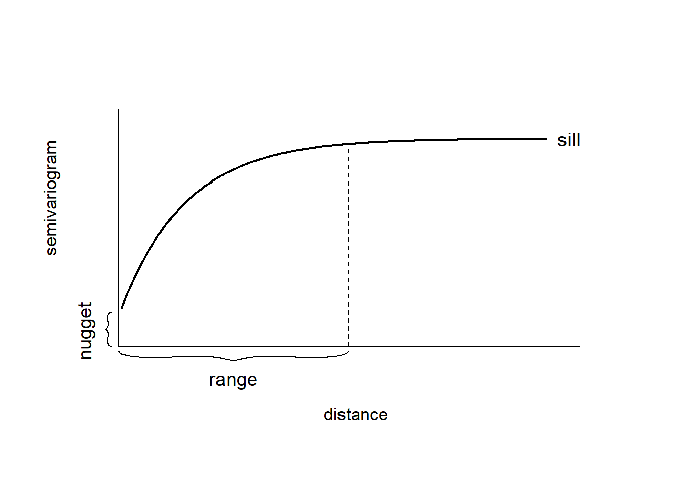
FIGURE 8.1: Typical semivariogram.

The empirical semivariogram can be used as exploratory tool to assess whether data present spatial correlation. Moreover, we can compare the empirical semivariogram with a Monte Carlo envelope of empirical semivariograms computed from random permutations of the data holding the locations fixed (Diggle and Ribeiro Jr. 2007). If the empirical semivariogram increases with distance and lies outside the Monte Carlo envelope, there is evidence of spatial correlation.

The covariance matrix of a GRF specifies its dependence structure and it is constructed from a covariance function. Common covariance functions are the exponential and Matérn models (Gelfand et al. 2010). For locations $\boldsymbol{s}_i$ and $\boldsymbol{s}_j \in \mathbb{R}^2$, the exponential covariance function is given by

\[\mbox{Cov}(Z(\boldsymbol{s}_i), Z(\boldsymbol{s}_j)) = \sigma^2 exp(- \kappa ||\boldsymbol{s}_i - \boldsymbol{s}_j ||),\]

where $||\boldsymbol{s}_i - \boldsymbol{s}_j ||$ denotes the distance between locations $\boldsymbol{s}_i$ and $\boldsymbol{s}_j$, $\sigma^2$ denotes the variance of the spatial field, and the parameter $\kappa > 0$ controls how fast the correlation decays with distance.

The Matérn family represents a very flexible class of covariance functions that appears naturally in many scientific fields (Guttorp and Gneiting 2006). The Matérn covariance function is defined as

\[\mbox{Cov}(Z(\boldsymbol{s}_i), Z(\boldsymbol{s}_j))=\frac{\sigma^2}{2^{\nu-1}\Gamma(\nu)}(\kappa ||\boldsymbol{s}_i - \boldsymbol{s}_j ||)^\nu K_\nu(\kappa ||\boldsymbol{s}_i - \boldsymbol{s}_j ||).\] Here, $\sigma^2$ denotes the marginal variance of the spatial field, and $K_\nu(\cdot)$ is the modified Bessel function of second kind and order $\nu>0$. The integer value of $\nu$ determines the mean square differentiability of the process and it is usually fixed since it is poorly identified in applications. For $\nu = 1/2$, the Matérn covariance function is equivalent to the exponential covariance function. $\kappa >0$ is related to the range $\rho$, the distance at which the correlation between two points is approximately 0. Specifically, $\rho = \sqrt{8\nu}/\kappa,$ and at this distance the spatial correlation is close to 0.1 (Cameletti et al. 2013). Examples of exponential and Matérn covariance functions are shown in Figure 8.2.

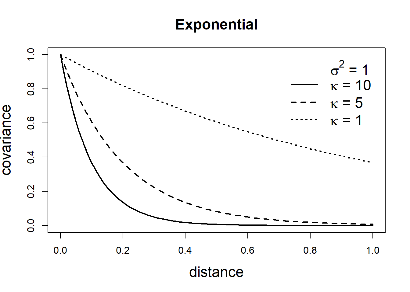
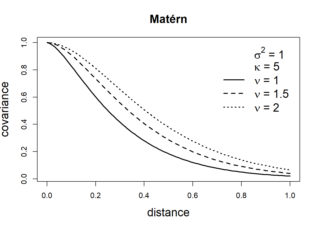
FIGURE 8.2: Covariance functions corresponding to exponential and Matérn models.

8.2 Stochastic partial differential equation approach

When geostatistical data are considered, we can often assume that there is a spatially continuous variable underlying the observations that can be modeled using a Gaussian random field. Then, we can use the stochastic partial differential equation approach (SPDE) implemented in the R-INLA package to fit a spatial model and predict the variable of interest at unsampled locations (Lindgren and Rue 2015). As shown in Whittle (1963), a GRF with a Matérn covariance matrix can be expressed as a solution to the following continuous domain SPDE:

\[(\kappa^2 - \Delta)^{\alpha/2}(\tau x(\boldsymbol{s})) = \mathcal{W}(\boldsymbol{s}).\]

Here, $x(\boldsymbol{s})$ is a GRF and $\mathcal{W}(\boldsymbol{s})$ is a Gaussian spatial white noise process. $\alpha$ controls the smoothness of the GRF, $\tau$ controls the variance, and $\kappa >0$ is a scale parameter. $\Delta$ is the Laplacian defined as $\sum_{i=1}^d \frac{\partial^2}{\partial x^2_i}$ where $d$ is the dimension of the spatial domain $D$.

The parameters of the Matérn covariance function and the SPDE are coupled as follows. The smoothness parameter $\nu$ of the Matérn covariance function is related to the SPDE through

\[\nu = \alpha - \frac{d}{2},\] and the marginal variance $\sigma^2$ is related to the SPDE through

\[\sigma^2 = \frac{\Gamma(\nu)}{\Gamma(\alpha)(4\pi)^{d/2}\kappa^{2\nu}\tau^2}.\]

For $d=2$ and $\nu=1/2$ which corresponds to the exponential covariance function, the parameter $\alpha = \nu + d/2 =1/2+1=3/2$. In the R-INLA package the default value is $\alpha = 2$, although options $0\leq \alpha < 2$ are also available.

An approximate solution of the SPDE can be found by using the Finite Element method. This method divides the spatial domain $D$ into a set of non-intersecting triangles leading to a triangulated mesh with $n$ nodes and $n$ basis functions. Basis functions $\psi_k(\cdot)$ are defined as piecewise linear functions on each triangle that is equal to 1 at vertex $k$, and equal to 0 at the other vertices. Then, the continuously indexed Gaussian field $x$ is represented as a discretely indexed Gaussian Markov random field (GMRF) by means of the finite basis functions defined on the triangulated mesh

\[x(\boldsymbol{s})=\sum_{k=1}^n \psi_k(\boldsymbol{s}) x_k,\] where $n$ is the number of vertices of the triangulation, $\psi_k(\cdot)$ denotes the piecewise linear basis functions, and $\{x_k\}$ are zero-mean Gaussian distributed weights.

The joint distribution of the weight vector is assigned a Gaussian distribution $\boldsymbol{x}=({x}_1,\ldots,{x}_n) \sim N(\boldsymbol{0}, \boldsymbol{Q}^{-1}(\tau, \kappa))$ that approximates the solution $x(\boldsymbol{s})$ of the SPDE in the mesh nodes, and the basis functions transform the approximation $x(\boldsymbol{s})$ from the mesh nodes to the other spatial locations of interest.

8.3 Spatial modeling of rainfall in Paraná, Brazil

In this example, we show how to predict rainfall in the state of Paraná, Brazil, using data from the geoR package (Ribeiro Jr et al. 2022). The data parana contains several objects with the average rainfall recorded over different years over the period May-June at 143 recording stations in Paraná. Specifically, parana$coords is a matrix with the coordinates of the recording stations, parana$data contains the rainfall values at the stations, and parana$border is a matrix with the coordinates defining the borders of Paraná. We can plot the rainfall values at each of the recording stations with the ggplot() function of the ggplot2 package as follows (Figure 8.3):

library(geoR)
library(ggplot2)

ggplot(data.frame(cbind(parana$coords, Rainfall = parana$data)))+
  geom_point(aes(east, north, color = Rainfall), size = 2) +
  coord_fixed(ratio = 1) +
  scale_color_gradient(low = "blue", high = "orange") +
  geom_path(data = data.frame(parana$border), aes(east, north)) +
  theme_bw()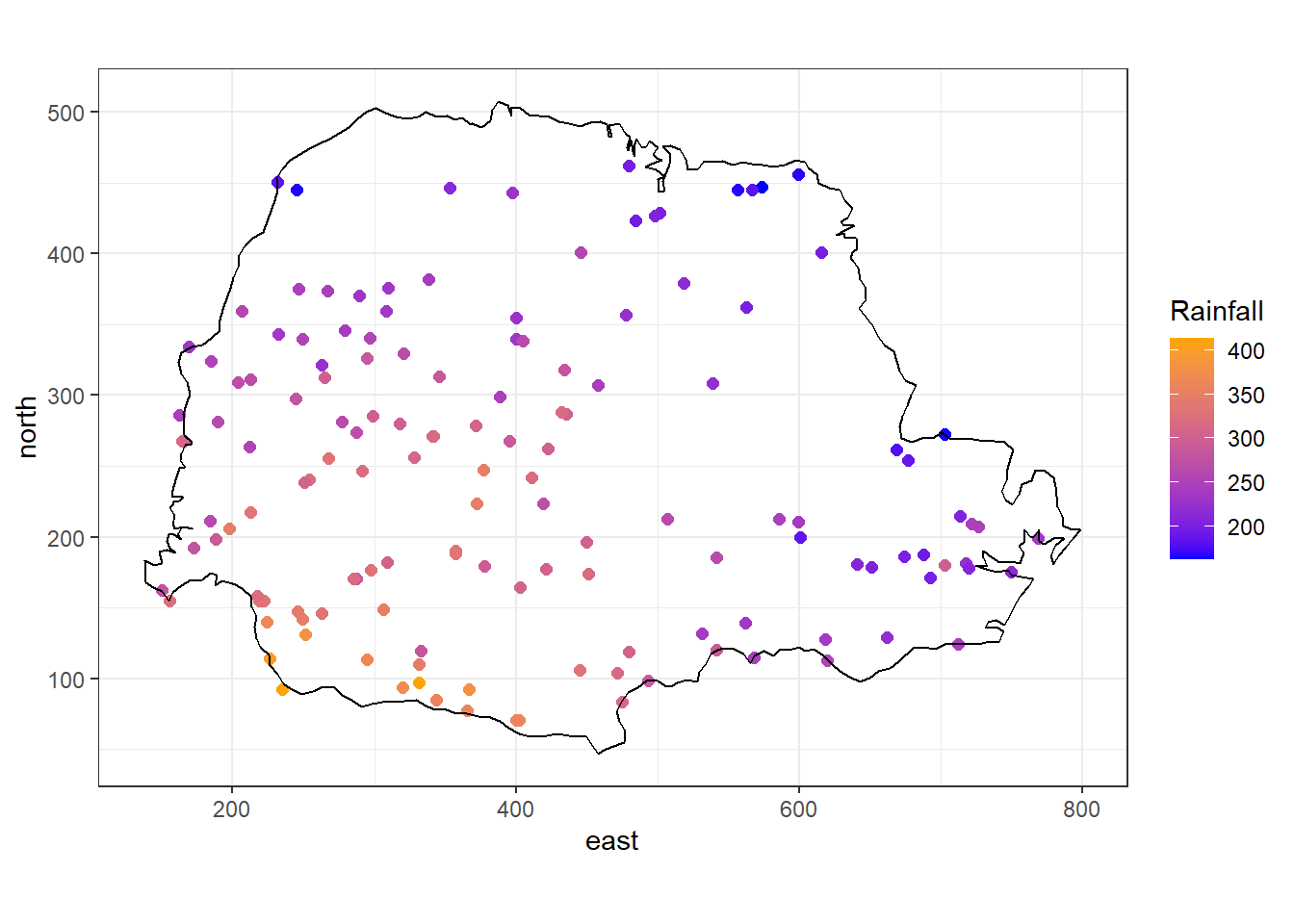

FIGURE 8.3: Average rainfall measured at 143 recording stations in Paraná state, Brazil.

8.3.1 Model

Rainfall values are available at the locations of the recording stations. However, rainfall occurs continuously in space and we can use a geostatistical model to predict rainfall values in other locations of Paraná. For example, we can assume that rainfall at location $\boldsymbol{s_i}$, $Y_i$, follows a Gaussian distribution with mean $\mu_i$ and variance $\sigma^2$, and the mean $\mu_i$ is expressed as the sum of an intercept $\beta_0$ and a spatially structured random effect that follows a zero-mean Gaussian process with Matérn covariance function:

\[Y_i \sim N(\mu_i, \sigma^2),\ i=1,2,\ldots,n,\]

\[\mu_i = \beta_0 + Z(\boldsymbol{s_i}).\]

Below we describe the steps to fit this model using the SPDE approach implemented in the R-INLA package.

8.3.2 Mesh construction

The SPDE approach approximates the continuous Gaussian field $Z(\cdot)$ as a discrete Gaussian Markov random field by means of a finite basis function defined on a triangulated mesh of the region of study. We can construct a triangulated mesh to perform this approximation with the inla.mesh.2d() function of the R-INLA package. The arguments of this function include:

loc: location coordinates that are used as initial mesh vertices,
boundary: object describing the boundary of the domain,
offset: distance that specifies the size of the inner and outer extensions around the data locations,
cutoff: minimum allowed distance between points. This is used to avoid building many small triangles around clustered locations,
max.edge: values denoting the maximum allowed triangle edge lengths in the region and in the extension.

In our example, we call inla.mesh.2d() setting loc equal to the matrix with the coordinates of the recording stations (coo). Then we specify offset = c(50, 100) to have an inner extension of size 50, and an outer extension of size 100 around the locations. We set cutoff = 1 to avoid building many small triangles where we have some very close points. Finally, we set max.edge = c(30, 60) to use small triangles within the region, and larger triangles in the extension. The triangulated mesh obtained is shown in Figure 8.4.

library(INLA)
coo <- parana$coords
summary(dist(coo))

##    Min. 1st Qu.  Median    Mean 3rd Qu.    Max. 
##       1     144     231     244     334     620

mesh <- inla.mesh.2d(
  loc = coo, offset = c(50, 100),
  cutoff = 1, max.edge = c(30, 60)
)
plot(mesh)
points(coo, col = "red")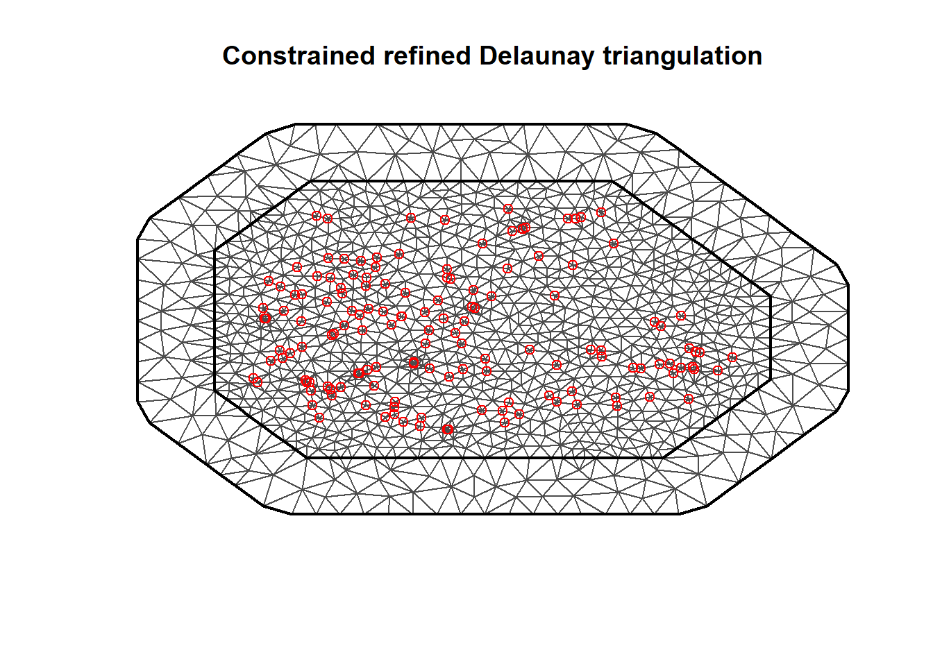

FIGURE 8.4: Triangulated mesh to build the SPDE model.

The number of vertices of the triangulated mesh can be seen by typing mesh$n.

mesh$n

## [1] 1189

It is also possible to construct the mesh using a boundary of the region of study. For example, we can construct a non-convex boundary for the coordinates using the inla.nonconvex.hull() function, and then pass it to inla.mesh.2d() to construct the mesh (Figure 8.5).

bnd <- inla.nonconvex.hull(coo)
meshb <- inla.mesh.2d(
  boundary = bnd, offset = c(50, 100),
  cutoff = 1, max.edge = c(30, 60)
)
plot(meshb)
points(coo, col = "red")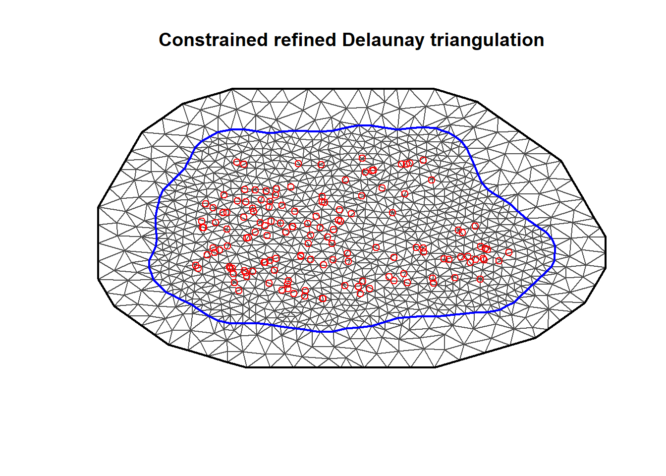

FIGURE 8.5: Non-convex triangulated mesh to build the SPDE model.

8.3.3 Building the SPDE model on the mesh

Now we use the inla.spde2.matern() function to build the SPDE model on the mesh passing mesh and alpha. Parameter alpha is related to the smoothness parameter of the process, namely, $\alpha=\nu+d/2$. In this example, we set the smoothness parameter $\nu$ equal to 1 and in the spatial case $d=2$ so alpha=1+2/2=2. We also set constr = TRUE to impose an integrate-to-zero constraint.

spde <- inla.spde2.matern(mesh = mesh, alpha = 2, constr = TRUE)

8.3.4 Index set

Then we generate the index set for the SPDE model. We do this with the function inla.spde.make.index() where we specify the name of the effect (s) and the number of vertices in the SPDE model (spde$n.spde).

indexs <- inla.spde.make.index("s", spde$n.spde)

8.3.5 Projection matrix

We need to construct a projection matrix $A$ to project the GRF from the observations to the triangulation vertices. The matrix $A$ has the number of rows equal to the number of observations, and the number of columns equal to the number of vertices of the triangulation. Row $i$ of $A$ corresponding to an observation at location $\boldsymbol{s}_i$ possibly has three non-zero values at the columns that correspond to the vertices of the triangle that contains the location. If $\boldsymbol{s}_i$ is within the triangle, these values are equal to the barycentric coordinates. That is, they are proportional to the areas of each of the three subtriangles defined by the location $\boldsymbol{s}_i$ and the triangle’s vertices, and sum to 1. If $\boldsymbol{s}_i$ is equal to a vertex of the triangle, row $i$ has just one non-zero value equal to 1 at the column that corresponds to the vertex. Intuitively, the value $Z(\boldsymbol{s})$ at a location that lies within one triangle is the projection of the plane formed by the triangle vertices weights at location $\boldsymbol{s}$.

An example of a projection matrix is given below. This projection matrix projects $n$ observations to $G$ triangulation vertices. The first row of the matrix corresponds to an observation with location that coincides with vertex number 3. The second and last rows correspond to observations with locations lying within triangles.

\[ A = \begin{bmatrix} A_{11} & A_{12} & A_{13} & \dots & A_{1G} \\ A_{21} & A_{22} & A_{23} & \dots & A_{2G} \\ \vdots & \vdots & \vdots & \ddots & \vdots \\ A_{n1} & A_{n2} & A_{n3} & \dots & A_{nG} \end{bmatrix} = \begin{bmatrix} 0 & 0 & 1 & \dots & 0 \\ A_{21} & A_{22} & 0 & \dots & A_{2G} \\ \vdots & \vdots & \vdots & \ddots & \vdots \\ A_{n1} & A_{n2} & A_{n3} & \dots & 0 \end{bmatrix} \]

Figure 8.6 shows a location $\boldsymbol{s}$ that lies within one of the triangles of a triangulated mesh. The value of the process $Z(\cdot)$ at $\boldsymbol{s}$ is expressed as a weighted average of the values of the process at the vertices of the triangle ($Z_1$, $Z_2$ and $Z_3$) and with weights equal to $T_1/T$, $T_2/T$ and $T_3/T$, where $T$ denotes the area of the big triangle that contains $\boldsymbol{s}$, and $T_1, T_2, T_3$ are the areas of the subtriangles.

\[Z(\boldsymbol{s}) \approx \frac{T_1}{T} Z_1 + \frac{T_2}{T} Z_2 + \frac{T_3}{T} Z_3.\]

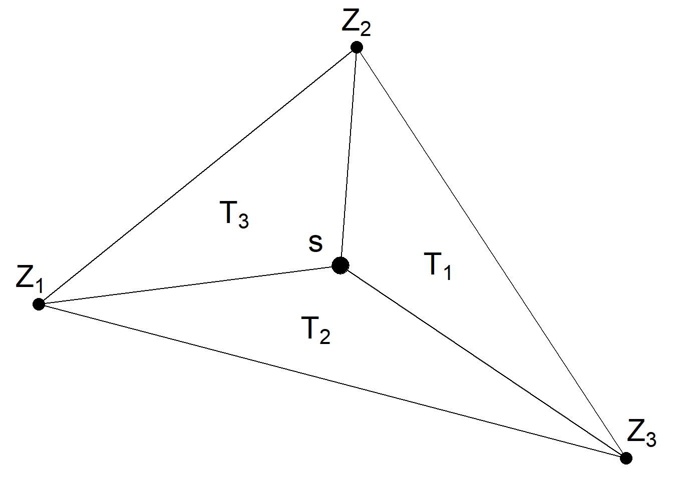
FIGURE 8.6: Triangle of a triangulated mesh.

R-INLA provides the inla.spde.make.A() function to easily construct a projection matrix $A$. We create the projection matrix of our example by using inla.spde.make.A() passing the triangulated mesh mesh and the coordinates coo.

A <- inla.spde.make.A(mesh = mesh, loc = coo)

We can type dim(A) to see $A$ has the number of rows equal to the number of observations, and the number of columns equal to the number of vertices of the mesh (mesh$n).

# dimension of the projection matrix
dim(A)

## [1]  143 1189

# number of observations
nrow(coo)

## [1] 143

# number of vertices of the triangulation
mesh$n

## [1] 1189

We can also see the elemens of each row sum to 1.

rowSums(A)

##   [1] 1 1 1 1 1 1 1 1 1 1 1 1 1 1 1 1 1 1 1 1 1 1 1 1 1
##  [26] 1 1 1 1 1 1 1 1 1 1 1 1 1 1 1 1 1 1 1 1 1 1 1 1 1
##  [51] 1 1 1 1 1 1 1 1 1 1 1 1 1 1 1 1 1 1 1 1 1 1 1 1 1
##  [76] 1 1 1 1 1 1 1 1 1 1 1 1 1 1 1 1 1 1 1 1 1 1 1 1 1
## [101] 1 1 1 1 1 1 1 1 1 1 1 1 1 1 1 1 1 1 1 1 1 1 1 1 1
## [126] 1 1 1 1 1 1 1 1 1 1 1 1 1 1 1 1 1 1

8.3.6 Prediction data

Now we construct a matrix with the coordinates of the locations where we will predict the rainfall values. First, we construct a grid called coop with $50 \times 50$ locations by using expand.grid() and combining vectors x and y which contain coordinates in the range of parana$border.

bb <- bbox(parana$border)
x <- seq(bb[1, "min"] - 1, bb[1, "max"] + 1, length.out = 50)
y <- seq(bb[2, "min"] - 1, bb[2, "max"] + 1, length.out = 50)
coop <- as.matrix(expand.grid(x, y))

Then we keep only the points of coop that lie within parana$border using the point.in.polygon() function of the sp package (Pebesma and Bivand 2024). The prediction locations are shown in Figure 8.7.

ind <- point.in.polygon(
  coop[, 1], coop[, 2],
  parana$border[, 1], parana$border[, 2]
)
coop <- coop[which(ind == 1), ]
plot(coop, asp = 1)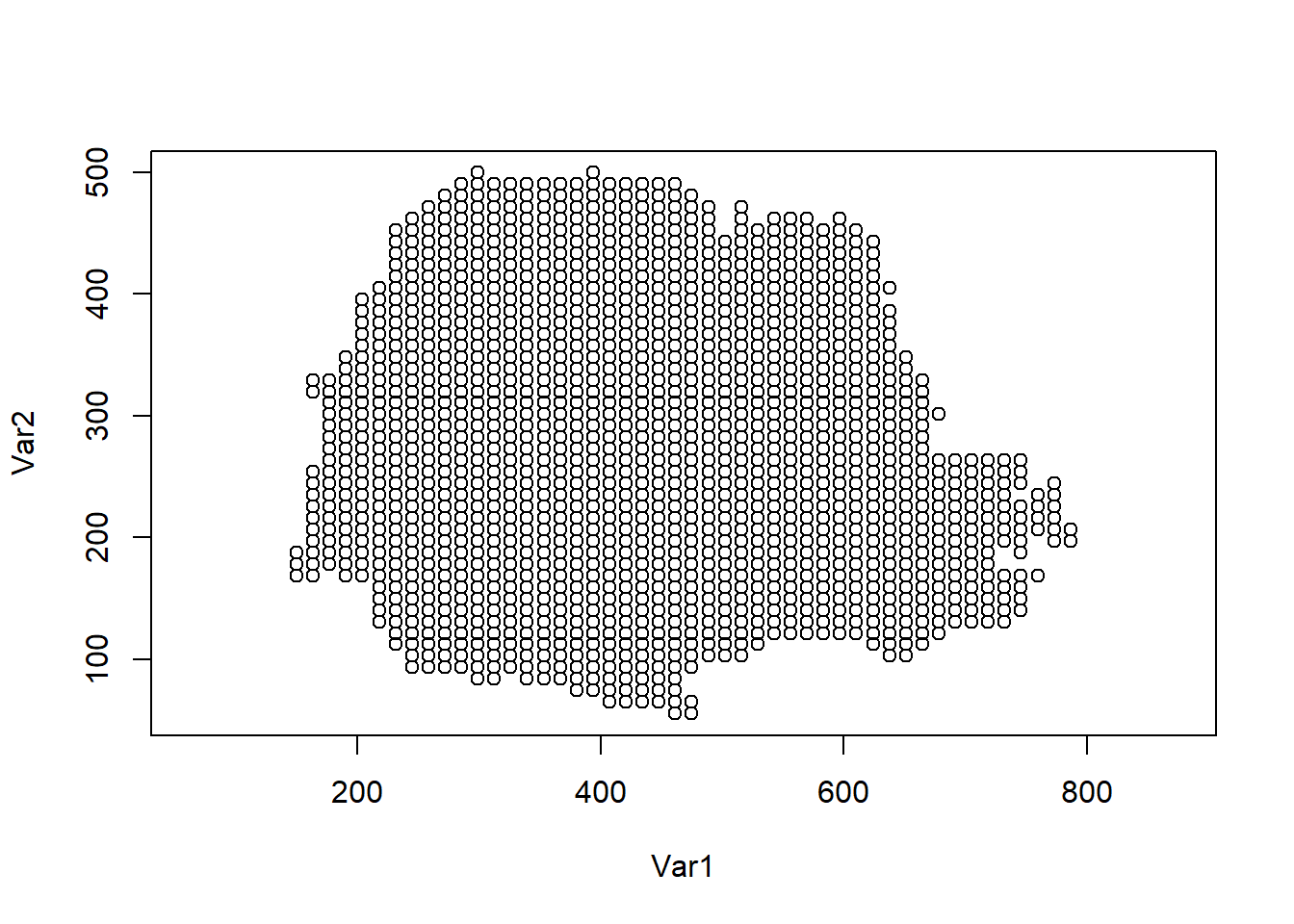

FIGURE 8.7: Prediction locations in Paraná state, Brazil.

We also create a projection matrix for the prediction locations using the inla.spde.make.A() function with arguments mesh and coop.

Ap <- inla.spde.make.A(mesh = mesh, loc = coop)
dim(Ap)

## [1] 1533 1189

8.3.7 Stack with data for estimation and prediction

Now we use the inla.stack() function to organize the data, effects, and projection matrices. We use the following arguments:

tag: string for identifying the data,
data: list of data vectors,
A: list of projection matrices,
effects: list with fixed and random effects.

We construct a stack called stk.e with data for estimation and we tag it with the string "est". The fixed effects are the intercept (b0) and the random effect is the spatial Gaussian Random Field (s). Therefore, in effects we pass a list with a data.frame with the fixed effects, and a list s containing the indices of the SPDE object (indexs). A is set to a list where the second element is A, the projection matrix for the random effects, and the first element is 1 to indicate the fixed effects are mapped one-to-one to the response. In data we specify the response vector. We also construct a stack for prediction called stk.p. This stack has tag "pred", the response vector is set to NA, and the data is specified at the prediction locations. Finally, we put stk.e and stk.p together in a full stack stk.full.

# stack for estimation stk.e
stk.e <- inla.stack(
  tag = "est",
  data = list(y = parana$data),
  A = list(1, A),
  effects = list(data.frame(b0 = rep(1, nrow(coo))), s = indexs)
)

# stack for prediction stk.p
stk.p <- inla.stack(
  tag = "pred",
  data = list(y = NA),
  A = list(1, Ap),
  effects = list(data.frame(b0 = rep(1, nrow(coop))), s = indexs)
)

# stk.full has stk.e and stk.p
stk.full <- inla.stack(stk.e, stk.p)

8.3.8 Model formula

The formula is specified by including the response in the left-hand side, and the fixed and random effects in the right-hand side. In the formula we remove the intercept (adding 0) and add it as a covariate term (adding b0).

formula <- y ~ 0 + b0 + f(s, model = spde)

8.3.9 `inla()` call

We fit the model by calling inla() and using the default priors in R-INLA. We specify the formula, data, and options. In control.predictor we set compute = TRUE to compute the posteriors of the predictions.

res <- inla(formula,
  data = inla.stack.data(stk.full),
  control.predictor = list(
    compute = TRUE,
    A = inla.stack.A(stk.full)
  )
)

8.3.10 Results

The data frame res$summary.fitted.values contains the mean, and the 2.5 and 97.5 percentiles of the fitted values. The indices of the rows corresponding to the predictions can be obtained with the inla.stack.index() function by passing stk.full and specifying the tag "pred".

index <- inla.stack.index(stk.full, tag = "pred")$data

We create the variable pred_mean with the posterior mean and variables pred_ll and pred_ul with the lower and upper limits of 95% credible intervals, respectively, as follows:

pred_mean <- res$summary.fitted.values[index, "mean"]
pred_ll <- res$summary.fitted.values[index, "0.025quant"]
pred_ul <- res$summary.fitted.values[index, "0.975quant"]

Now, we create maps of the predicted rainfall values (Figure 8.8). First, we construct a data frame with the prediction coordinates, and the means and lower upper limits of 95% credible intervals of the predictions.

dpm <- rbind(
  data.frame(
    east = coop[, 1], north = coop[, 2],
    value = pred_mean, variable = "pred_mean"
  ),
  data.frame(
    east = coop[, 1], north = coop[, 2],
    value = pred_ll, variable = "pred_ll"
  ),
  data.frame(
    east = coop[, 1], north = coop[, 2],
    value = pred_ul, variable = "pred_ul"
  )
)
dpm$variable <- as.factor(dpm$variable)

We create the maps using ggplot(). We use geom_tile() to plot the rainfall predictions in cells, and facet_wrap() to show the three maps in the same plot. We also use coord_fixed(ratio = 1) to ensure that one unit on the x-axis is the same length as one unit on the y-axis of the map. Finally, we use scale_fill_gradient() to specify a color scale that creates a sequential gradient between the color blue (low) and orange (high).

ggplot(dpm) + geom_tile(aes(east, north, fill = value)) +
  facet_wrap(~variable, nrow = 1) +
  coord_fixed(ratio = 1) +
  scale_fill_gradient(
    name = "Rainfall",
    low = "blue", high = "orange"
  ) +
  theme_bw()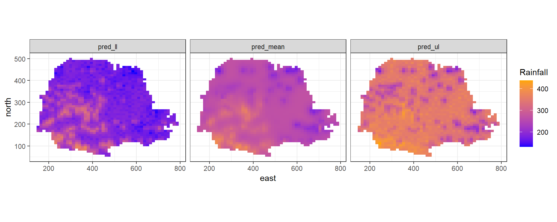

FIGURE 8.8: Rainfall predictions and lower and upper limits of 95% CI in Paraná state, Brazil.

8.3.11 Projecting the spatial field

Vectors res$summary.random$s$mean and res$summary.random$s$sd contain the posterior mean and the posterior standard deviation, respectively, of the spatial field at the mesh nodes. We can project these values at different locations by computing a projection matrix for the new locations and then multiplying the projection matrix by the spatial field values. For example, we can compute the posterior mean of the spatial field at locations in matrix newloc as follows:

newloc <- cbind(c(219, 678, 818), c(20, 20, 160))
Aproj <- inla.spde.make.A(mesh, loc = newloc)
Aproj %*% res$summary.random$s$mean

## 3 x 1 Matrix of class "dgeMatrix"
##          [,1]
## [1,] -1.64861
## [2,] -0.05843
## [3,]  0.92691

We can also project the spatial field values at different locations by using the inla.mesh.projector() and inla.mesh.project() functions. First, we need to use the inla.mesh.projector() function to compute a projection matrix for the new locations. We can either specify the locations in the argument loc, or we can compute the locations on a grid by specifying arguments xlim, ylim and dims. For example, we use inla.mesh.projector() to compute a projection matrix for 300 x 300 locations on a grid that covers the mesh region.

rang <- apply(mesh$loc[, c(1, 2)], 2, range)
proj <- inla.mesh.projector(mesh,
  xlim = rang[, 1], ylim = rang[, 2],
  dims = c(300, 300)
)

Then, we use the inla.mesh.project() function to project the posterior mean and the posterior standard deviation of the spatial field calculated at the mesh nodes to the grid locations.

mean_s <- inla.mesh.project(proj, res$summary.random$s$mean)
sd_s <- inla.mesh.project(proj, res$summary.random$s$sd)

We can plot the projected values using the ggplot2 package. First, we create a data frame with the coordinates of the grid locations and the spatial field values. The coordinates of the grid locations can be obtained by combining proj$x and proj$y using the expand.grid() function. The values of the posterior mean of the spatial field are in matrix mean_s, and the values of the posterior standard deviation of the spatial field are in matrix sd_s.

df <- expand.grid(x = proj$x, y = proj$y)
df$mean_s <- as.vector(mean_s)
df$sd_s <- as.vector(sd_s)

Finally, we use ggplot() and geom_raster() to create maps with the spatial field values. We plot the maps side-by-side on a grid by using the plot_grid() function of the cowplot package (Wilke 2020) (Figure 8.9).

library(viridis)
library(cowplot)

gmean <- ggplot(df, aes(x = x, y = y, fill = mean_s)) +
  geom_raster() +
  scale_fill_viridis(na.value = "transparent") +
  coord_fixed(ratio = 1) + theme_bw()

gsd <- ggplot(df, aes(x = x, y = y, fill = sd_s)) +
  geom_raster() +
  scale_fill_viridis(na.value = "transparent") +
  coord_fixed(ratio = 1) + theme_bw()

plot_grid(gmean, gsd)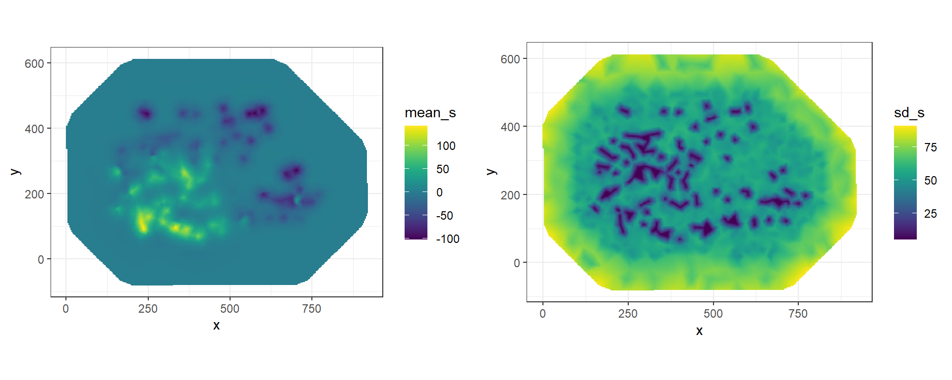

FIGURE 8.9: Posterior mean and posterior standard deviation of the spatial field projected on a grid.

8.4 Disease mapping with geostatistical data

In low- and middle- income countries, disease prevalence surveys are usually conducted to quantify the risk of diseases such as malaria and tuberculosis, and to inform prevention and control interventions. Prevalence surveys provide disease information only at specific locations; however, disease risk is a spatially continuous phenomenon and local predictions are needed to be able to direct resources where they are most needed. Model-based geostatistics can be used with this type of data to make predictions at unsampled locations and construct a spatially continuous surface of disease risk (Diggle and Ribeiro Jr. 2007). These models describe the variability in the response variable as a function of factors known to affect disease transmission such as temperature, precipitation or humidity, and spatial effects that account for residual spatial autocorrelation.

When data are available at a set of locations $\boldsymbol{s}_i$, $i = 1, \ldots, n$, we can predict disease prevalence by assuming that conditional on the true prevalence $P(\boldsymbol{s}_i)$ at location $\boldsymbol{s}_i$, the number of positive results $Y_i$ out of $N_i$ people sampled follows a binomial distribution, and the logit of the prevalence is expressed as a sum of covariates and a spatial random effect:

\[Y_i|P(\boldsymbol{s}_i) \sim Binomial(N_i, P(\boldsymbol{s}_i)),\]

\[logit(P(\boldsymbol{s}_i)) = \log\left(\frac{P(\boldsymbol{s}_i)}{1-P(\boldsymbol{s}_i)}\right) = \boldsymbol{d}_i \boldsymbol{\beta} + Z(\boldsymbol{s}_i).\]

Here, $\boldsymbol{d}_i = (1, d_{i1}, \ldots, d_{ip})$ is the vector of the intercept and $p$ covariates at location $\boldsymbol{s}_i$, $\boldsymbol{\beta} = (\beta_0, \beta_1, \ldots, \beta_p)'$ is the coefficient vector, and $Z(\cdot)$ is a spatially structured random effect which follows a zero-mean Gaussian process with Matérn covariance function. Coefficient $\beta_j$, $j=1,\ldots,p$, can be interpreted as the change in the log-odds associated with one unit increase in covariate $d_j$, holding all other covariates constant. Thus, $exp(\beta_j)$ is the odds ratio and for a one unit increase in covariate $d_j$ the odds increase by a factor of $exp(\beta_j)$, holding all other covariates constant.

This model can be fitted with the SPDE approach implemented in the R-INLA package. First, we construct a triangulated mesh and a projection matrix $A$ to project the Gaussian random field from the observations to the vertices of the triangulated mesh. Then, we define a formula that relates the number of positive results (y) as a sum of covariates (cov1 + ... + covn) and a random effect that is specified using the f() function with arguments the index variable s and the model spde.

formula <- y ~ cov1 + ... + covn + f(s, model = spde)

Finally, we construct a stack with the data and the projection matrix, and execute the inla() function where we specify the formula, the family (binomial), the number of trials, the data, and the projection matrix.

res <- inla(formula,
  family = "binomial", Ntrials = numtrials,
  data = inla.stack.data(stk.full),
  control.predictor = list(A = inla.stack.A(stk.full))
)

Similarly, spatio-temporal models can be used to model spatio-temporal variation of disease. In these settings, we can assume that the number of people tested positive $Y_{it}$ out of $N_{it}$ people sampled at location $\boldsymbol{s}_i$ and time $t$ follows a binomial distribution:

\[Y_{it}|P(\boldsymbol{s}_i, t) \sim Binomial(N_{it}, P(\boldsymbol{s}_i, t)),\]

and the logit of the prevalence is expressed as

\[logit(P(\boldsymbol{s}_i, t)) = \boldsymbol{d}_{it} \boldsymbol{\beta} + \xi(\boldsymbol{s}_i, t),\]

where $\boldsymbol{d}_{it} \boldsymbol{\beta}$ are the fixed effects, and $\xi(\boldsymbol{s}_i, t)$ denotes a spatio-temporal random effect. R-INLA permits to fit models where $\xi(\boldsymbol{s}_i, t)$ is expressed as

\[\xi(\boldsymbol{s}_i, t) = a \xi(\boldsymbol{s}_i, t-1) + w(\boldsymbol{s}_i, t),\] where $|a|<1$ and $\xi(\boldsymbol{s}_i, 1)$ follows a stationary distribution of a first-order autoregressive process (AR1), namely, $N(0, \sigma^2_w/(1-a^2))$. Each $w(\boldsymbol{s}_i, t)$ follows a zero-mean Gaussian distribution temporally independent but spatially dependent at each time. In R-INLA the formula of this model can be written as

formula <- y ~ cov1 + ... + covn +
  f(s, model = spde,
    group = s.group, control.group = list(model = "ar1")
  )

Here, y is the number of positive results and cov1 + ... + covn is the sum of covariates. The random effect is specified with the f() function with index variable s, model spde, group equal to the indices of the times, and control.group = list(model = "ar1"). This indicates that observations are related in time according to an AR1 model and depend on a spde model in space. Then, we can execute the inla() function where we provide the formula, the family (binomial), the number of trials, the data, and the projection matrix.

res <- inla(formula,
  family = "binomial", Ntrials = numtrials,
  data = inla.stack.data(stk.full),
  control.predictor = list(A = inla.stack.A(stk.full))
)

Note that spatial and spatio-temporal geostatistical models can be used to model other types of outcomes such as Gaussian or count data using appropriate distributions from an exponential family, and suitable link functions such as identity in case of Gaussian data and the logarithm in case of Poisson data. Moreover, models can be extended by including random effects that can deal with other sources of variability. Chapters 9 and 10 present further examples that show how to fit and interpret spatial and spatio-temporal geostatistical models in different settings.

7 Spatio-temporal modeling of areal data. Lung cancer in Ohio

9 Spatial modeling of geostatistical data. Malaria in The Gambia